Introduction to Ratio Analysis
Ratio Analysis
Ratio analysis is the assessment of the proportionate relationship, in time and amplitude, of one wave to another. In discerning the working of the Golden Ratio in the five up and three down movement of the stock market cycle, one might anticipate that on completion of any bull phase, the ensuing correction would be three-fifths of the previous rise in both time and amplitude. Such simplicity is seldom seen. However, the underlying tendency of the market to conform to relationships suggested by the Golden Ratio is always present and helps generate the right look for each wave.
The study of wave amplitude relationships in the stock market can often lead to such startling discoveries that some Elliott Wave practitioners have become almost obsessive about its importance. Although Fibonacci time ratios are far less common, years of plotting the averages have convinced the authors that the amplitude (measured either arithmetically or in percentage terms) of virtually every wave is related to the amplitude of an adjacent, alternate and/or component wave by one of the ratios between Fibonacci numbers. However, we shall endeavor to present the evidence and let it stand or fall on its own merit.
The first evidence we found of the application of time and amplitude ratios in the stock market comes from, of all suitable sources, the works of the great Dow Theorist, Robert Rhea. In 1936, Rhea, in his book The Story of the Averages, compiled a consolidated summary of market data covering nine Dow Theory bull markets and nine bear markets spanning a thirty-six year time period from 1896 to 1932. He had this to say about why he felt it was necessary to present the data despite the fact that no use for it was immediately apparent:
Whether or not [this review of the averages] has contributed anything to the sum total of financial history, I feel certain that the statistical data presented will save other students many months of work.... Consequently, it seemed best to record all the statistical data we had collected rather than merely that portion which appeared to be useful.... The figures presented under this heading probably have little value as a factor in estimating the probable extent of future movements; nevertheless, as a part of a general study of the averages, the treatment is worthy of consideration.
One of the observations was this one:
The footings of the tabulation shown above (considering only the industrial average) show that the nine bull and bear markets covered in this review extended over 13,115 calendar days. Bull markets were in progress 8,143 days, while the remaining 4,972 days were in bear markets. The relationship between these figures tends to show that bear markets run 61.1 percent of the time required for bull periods.
And finally,
Column 1 shows the sum of all primary movements in each bull (or bear) market. It is obvious that such a figure is considerably greater than the net difference between the highest and lowest figures of any bull market. For example, the bull market discussed in Chapter II started (for Industrials) at 29.64 and ended at 76.04, and the difference, or net advance, was 46.40 points. Now this advance was staged in four primary swings of 14.44, 17.33, 18.97, and 24.48 points respectively. The sum of these advances is 75.22, which is the figure shown in Column 1. If the net advance, 46.40, is divided into the sum of advances, 75.22, the result is 1.621, which gives the percent shown in Column 1. Assume that two investors were infallible in their market operations, and that one bought stocks at the low point of the bull market and retained them until the high day of that market before selling. Call his gain 100 percent. Now assume that the other investor bought at the bottom, sold out at the top of each primary swing, and repurchased the same stocks at the bottom of each secondary reaction — his profit would be 162.1, compared with 100 realized by the first investor. Thus the total of secondary reactions retraced 62.1 percent of the net advance. [Emphasis added.]
So in 1936 Robert Rhea discovered, without knowing it, the Fibonacci ratio and its function relating bull phases to bear in both time and amplitude. Fortunately, he felt that there was value in presenting data that had no immediate practical utility, but that might be useful at some future date. Similarly, we feel that there is much to learn on the ratio front and our introduction, which merely scratches the surface, could be valuable in leading some future analyst to answer questions we have not even thought to ask. Ratio analysis has revealed a number of precise price relationships that occur often among waves. There are two categories of relationships: retracements and multiples.
Retracements
Occasionally, a correction retraces a Fibonacci percentage of the preceding wave. As illustrated in Figure 4-1, sharp corrections tend more often to retrace 61.8% or 50% of the previous wave, particularly when they occur as wave 2 of an impulse wave, wave B of a larger zigzag, or wave X in a multiple zigzag. Sideways corrections tend more often to retrace 38.2% of the previous impulse wave, particularly when they occur as wave 4, as shown in Figure 4-2.
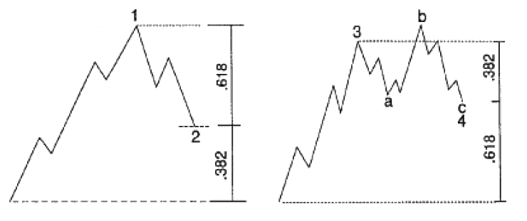
Figure 4-1 and Figure 4-2
Retracements come in all sizes. The ratios shown in Figures 4-1 and 4-2 are merely tendencies, yet that is where most analysts place an inordinate focus because measuring retracements is easy. Far more precise and reliable, however, are relationships between alternate waves, or lengths unfolding in the same direction, as explained in the next section.