Fibonacci Time Sequences
There is no sure way of using the time factor by itself in forecasting. Frequently, however, time relationships based on the Fibonacci sequence go beyond an exercise in numerology and seem to fit wave spans with remarkable accuracy, giving the analyst added perspective. Elliott said that the time factor often "conforms to the pattern" and therein lies its significance. In wave analysis, Fibonacci time periods serve to indicate possible times for a turn, especially if they coincide with price targets and wave counts.
In Nature's Law, Elliott gave the following examples of Fibonacci time spans between important turning points in the market:
1921 to 1929 (8 years)
July 1921 to November 1928 (89 months)
September 1929 to July 1932 (34 months)
July 1932 to July 1933 (13 months)
July 1933 to July 1934 (13 months)
July 1934 to March 1937 (34 months)
July 1932 to March 1937 (5 years)
March 1937 to March 1938 (13 months)
1929 to 1942 (13 years)
In Dow Theory Letters on November 21, 1973, Richard Russell gave some additional examples of Fibonacci time periods:
1907 panic low to 1962 panic low (55 years)
1949 major bottom to 1962 panic low (13 years)
1921 recession low to 1942 recession low (21 years)
January 1960 top to October 1962 bottom (34 months)
Taken in toto, these distances appear to be a bit more than coincidence.
Walter E. White, in his 1968 monograph on the Elliott Wave Principle, concluded that "the next important low point may be in 1970." As substantiation, he pointed out the following Fibonacci sequence: 1949 + 21 = 1970; 1957 + 13 = 1970; 1962 + 8 = 1970; 1965 + 5 = 1970. May 1970, of course, marked the low point of the most vicious slide in thirty years.
The progression of years from the 1928 (possible orthodox) and 1929 (nominal) high of the last Supercycle produces a remarkable Fibonacci sequence as well:
1929 + 3 = 1932 bear market bottom
1929 + 5 = 1934 correction bottom
1929 + 8 = 1937 bull market top
1929 + 13 = 1942 bear market bottom
1928 + 21 = 1949 bear market bottom
1928 + 34 = 1962 crash bottom
1928 + 55 = 1982 major bottom (1 year off)
A similar series has begun at the 1965 (possible orthodox) and 1966 (nominal) highs of the third Cycle wave of the current Supercycle:
1965 + 1 = 1966 nominal high
1965 + 2 = 1967 reaction low
1965 + 3 = 1968 blowoff peak for secondaries
1965 + 5 = 1970 crash low
1966 + 8 = 1974 bear market bottom
1966 + 13 = 1979 low for 9.2 and 4.5 year cycles
1966 + 21 = 1987 high, low and crash
In applying Fibonacci time periods to the pattern of the market, Bolton noted that time "permutations tend to become infinite" and that time "periods will produce tops to bottoms, tops to tops, bottoms to bottoms or bottoms to tops." Despite this reservation, he successfully indicated within the same book, which was published in 1960, that 1962 or 1963, based on the Fibonacci sequence, could produce an important turning point. 1962, as we now know, saw a vicious bear market and the low of Primary wave [4], which preceded a virtually uninterrupted advance lasting nearly four years.
In addition to this type of time sequence analysis, the time relationship between bull and bear as discovered by Robert Rhea has proved useful in forecasting. Robert Prechter, in writing for Merrill Lynch, noted in March 1978 that "April 17 marks the day on which the A-B-C decline would consume 1931 market hours, or .618 times the 3124 market hours in the advance of waves (1), (2) and (3)." Friday, April 14 marked the upside breakout from the lethargic inverse head and shoulders pattern on the Dow, and Monday, April 17 was the explosive day of record volume, 63.5 million shares. While this time projection did not coincide with the low, it did mark the exact day when the psychological pressure of the preceding bear was lifted from the market.
Benner's Theory
Samuel T. Benner had been an ironworks manufacturer until the post Civil War panic of 1873 ruined him financially. He turned to wheat farming in Ohio and took up the statistical study of price movements as a hobby to find, if possible, the answer to the recurring ups and downs in business. In 1875, Benner wrote a book entitled Business Prophecies of the Future Ups and Downs in Prices. The forecasts contained in his book are based mainly on cycles in pig iron prices and the recurrence of financial panics over a fairly considerable period of years. Benner's forecasts proved remarkably accurate for many years, and he established an enviable record for himself as a statistician and forecaster. Even today, Benner's charts are of interest to students of cycles and are occasionally seen in print, sometimes without due credit to the originator.
Benner noted that the highs of business tend to follow a repeating 8-9-10 yearly pattern. If we apply this pattern to high points in the Dow Jones Industrial Average over the past seventy-five years starting with 1902, we get the following results. These dates are not projections based on Benner's forecasts from earlier years, but are only an application of the 8-9-10 repeating pattern applied in retrospect.
| Year | Interval | Market Highs |
|---|---|---|
| 1902 | April 24, 1902 | |
| 1910 | 8 | January 2, 1910 |
| 1919 | 9 | November 3, 1919 |
| 1929 | 10 | September 3, 1929 |
| 1937 | 8 | March 10, 1937 |
| 1946 | 9 | May 29, 1946 |
| 1956 | 10 | April 6, 1956 |
| 1964 | 8 | February 4, 1965 |
| 1973 | 9 | January 11, 1973 |
With respect to economic low points, Benner noted two series of time sequences indicating that recessions (bad times) and depressions (panics) tend to alternate (not surprising, given Elliott's rule of alternation). In commenting on panics, Benner observed that 1819, 1837, 1857 and 1873 were panic years and showed them in his original "panic" chart to reflect a repeating 16-18-20 pattern, resulting in an irregular periodicity of these recurring events. Although he applied a 20-18-16 series to recessions, or "bad times," less serious stock market lows seem rather to follow the same 16-18-20 pattern as do major panic lows. By applying the 16-18-20 series to the alternating stock market lows, we get an accurate fit, as the Benner-Fibonacci Cycle Chart (Figure 4-17), first published in the 1967 supplement to the Bank Credit Analyst, graphically illustrates.
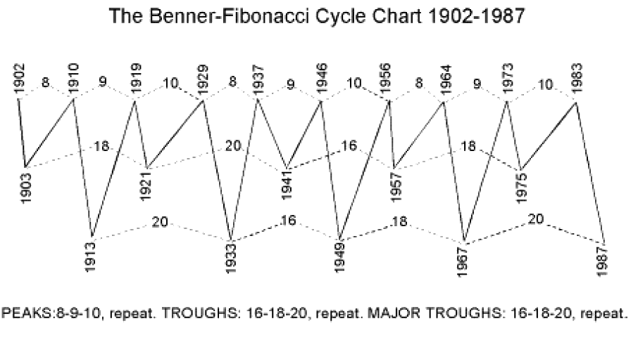
Figure 4-17
Note that the last time the cycle configuration was the same as the present was the period of the 1920s, paralleling the last occurrence of a fifth Elliott wave of Cycle degree.
This formula, based upon Benner's idea of repeating series for tops and bottoms, has worked reasonably well for most of this century. Whether the pattern will always reflect future highs is another question. These are fixed cycles, after all, not Elliott. Nevertheless, in our search for the reason for its satisfactory fit with reality, we find that Benner's theory conforms reasonably closely to the Fibonacci sequence in that the repeating series of 8-9-10 produces Fibonacci numbers up to the number 377, allowing for a marginal difference of one point.
Our conclusion is that Benner's theory, which is based on different rotating time periods for bottoms and tops rather than constant repetitive periodicities, falls within the framework of the Fibonacci sequence. Had we no experience with the approach, we might not have mentioned it, but it has proved useful in the past when applied in conjunction with a knowledge of Elliott Wave progression. A.J. Frost applied Benner's concept in late 1964 to make the inconceivable (at the time) prediction that stock prices were doomed to move essentially sideways for the next ten years, raching a high in 1973 at about 1000 DJIA and a low in the 500 to 600 zone in late 1974 or early 1975. A letter sent by Forst to Hamilton Bolton at the time is reproduced here. Figure 4-18 is a reproduction of the accompanying chart, complete with notes. As the letter was dated December 10, 1964, it represents yet another long term Elliott prediction which turned out to be more fact than fancy.
Although we have been able to codify ratio analysis substantially as described in the first half of this chapter, there appear to be many ways that the Fibonacci ratio is manifest in the stock market. The approaches suggested here are merely carrots to whet the appetite of prospective analysts and set them on the right track. Parts of the following chapters further explore the use of ratio analysis and give perspective on its complexity, accuracy and applicability. Additional detailed examples are presented in the Lessons 32 through 34. Obviously, the key is there. All that remains is to discover how many doors it will unlock.